The following is part of a series of posts about 2026 summer intern projects—for more, see “What the interns have wrought, special jumbo 2026 edition”

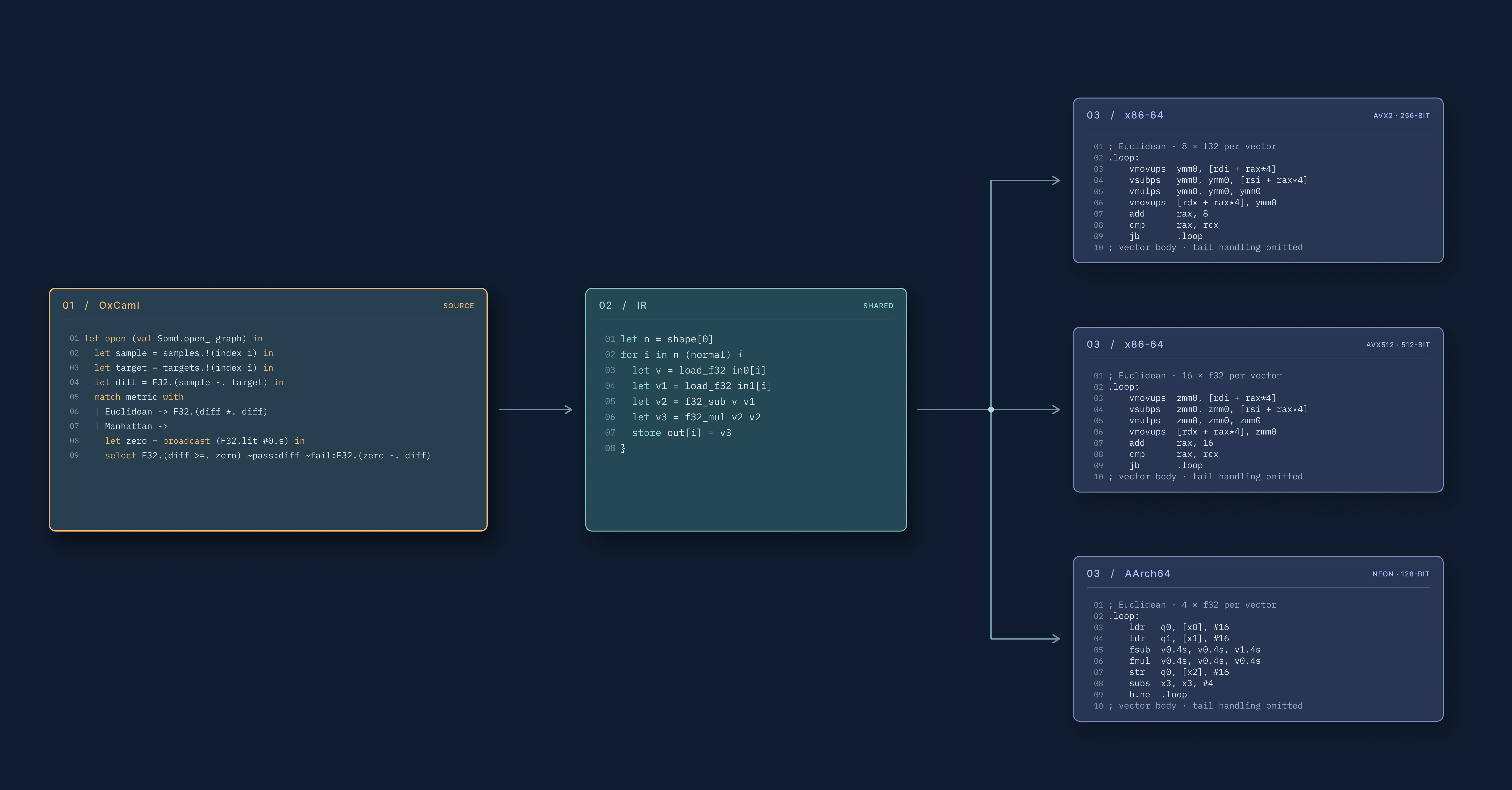
We have a lot of performance-critical SIMD code (single-instruction, multiple-data) running on CPUs across the firm. These are highly parallel programs where you run the same computation across arrays of data, in our case for options pricing or for low-latency risk checks. Because OCaml hasn’t historically exposed SIMD instructions, these programs often involve an inner loop written in fairly esoteric C. Writing these loops requires implementers to think carefully about hardware, and doing performance tuning, such as modifying unroll factors or vector widths, can require major changes to the code. Moreover, these programs are constrained to a specific instruction set. If we were to target a different architecture or a newer processor, we’d have to rewrite the program.

For his summer internship, Sai Konkimalla built a compiler for a domain specific language (DSL) that makes SIMD more ergonomic and widely accessible. The compiler takes advantage of OxCaml features that were only very recently added to the language, such as runtime metaprogramming, to enable users to write a kernel just once as a regular-ish OxCaml function, then compile and run it on multiple architectures.

Single Program, Multiple Data

To help solve the problem of SIMD code being rather difficult to write and maintain, our DSL uses the SPMD, or “single program, multiple data” programming model. As opposed to SIMD intrinsics, SPMD is higher level and not tied to a specific instruction set. We might normally think of higher-level languages as slower, but with SPMD, a higher level of abstraction lets the compiler make better decisions about how to optimally use the underlying hardware. This ability can lead to significantly faster code.

SPMD was popularized by CUDA (for Nvidia GPUs) and ISPC (for Intel CPUs). In this model, you write a program describing what happens at each index of a loop, then the compiler converts it into a parallel computation. For example, in CUDA:

__global__ void kernel(const float* x, float* out, int n) {
    int idx = blockIdx.x * blockDim.x + threadIdx.x;
    if (idx < n) {
        out[idx] = 2.0f * x[idx] + idx;
    }
}

Notice how there’s no loop here: you only define the loop body, and the compiler decides how to run it. In CUDA, when you launch a kernel on a GPU, you can declare how many blocks of threads to run and the GPU will schedule them accordingly.

In ISPC, foreach also abstracts away how the loop is actually executed:

export void kernel(uniform float x[], uniform float out[], uniform int n) {
    foreach (i = 0 ... n) {
        out[i] = 2.0f * x[i] + i;
    }
}

In both cases, the compiler translates the code into low-level SIMD instructions. Not specifying the exact instructions also means SPMD programs can benefit from future hardware improvements. If we get a new, faster CPU with a different instruction set, the SPMD compiler can seamlessly compile existing code to it.

A quick overview of the DSL

Let’s go over an example of the DSL that Sai implemented. We start by defining the kernel’s signature, including its output type, input types, and the dimension of the output:

Spmd.Kernel.create
 F32           (* output element type *)
 [ F32; F32 ]  (* input slice types   *)
 [ () ]        (* one output dimension *)
 (fun graph [ x; scale] [ Dim i ] -> exclave_
   ...)

In this example, we’re writing a kernel that takes in two F32 slices and returns one F32 slice.

Future work on a ppx syntax extension will make it possible to rewrite the above simply as:

let%spmd kernel (x : f32 slice) (scale : f32) (i : dim) : f32 =

Next, we write the actual computation:

Spmd.Kernel.create
  F32           (* output element type *)
  [ F32; F32 ]  (* input slice types   *)
  [ () ]        (* one output dimension *)
  (fun graph [ x; scale ] [ Dim i ] -> exclave_
     let open (val Spmd.open_ graph) in
     let i = index i in
     F32.((x.!(i) *. broadcast scale.!(I32.lit #0l)) +. of_i32 i))

Note the let open (val Spmd.open_ graph) in. This brings the DSL operations which construct a computational graph into scope. You can think of the graph value as proof that you’re in the graph-construction phase, not the runtime of the generated program. (Bonsai uses a similar trick for creating its incremental graph.)

Like CUDA, we don’t write the kernel as a loop. Instead, the developer writes a function that computes a single entry of the output slice, and the SPMD compiler generates code to loop over the output slice and compute the value at each index.

You may wonder why we loop over the output and not the inputs. Looping over the output is easier to model because each iteration writes to exactly one location, so iterations can be easily vectorized, reordered, or parallelized. If we were to loop over the inputs, different iterations could write to the same output entry. The compiler would then have to reason about whether the writes could be re-ordered. By guaranteeing that each output entry is written exactly once, we can avoid this complexity.

Where runtime metaprogramming comes in

One wrinkle with Sai’s project is that we wanted to execute the SPMD compiler at runtime. Runtime compilation (often called just-in-time or JIT compilation) is when the compiler generates code while the program is running. This gives us two main advantages: we don’t have to worry about building for all potential target architectures at compile time, and we can use data obtained at runtime for optimizations.

That latter point is especially important for generating high-performance code. When executing at runtime, the compiler has more data that it can use to optimize the code than it would when executing ahead-of-time. For example, our compiler can use runtime data to compile away branch instructions, which can slow down execution by consuming CPU resources.

To implement our JIT compiler, we used runtime metaprogramming, a feature that lets us generate, compile, and evaluate OxCaml code at runtime by using the OxCaml compiler as a library. As far as we know, Sai’s project was the first real program at Jane Street to use it. (He discovered some bugs in its implementation and helped report/reproduce them for the OxCaml team.)

Let’s take a look at an example that illustrates the power of compiling at runtime. In this code, we match on the metric to choose which algorithm to execute:

type metric =
  | Euclidean
  | Manhattan

let measure ~metric =
  Spmd.Kernel.create
    F32
    [ F32; F32 ]
    [ () ]
    (fun graph [ samples; targets ] [ Dim i ] -> exclave_
       let open (val Spmd.open_ graph) in
       let sample = samples.!(index i) in
       let target = targets.!(index i) in
       let diff = F32.(sample -. target) in
       match metric with
       | Euclidean -> F32.(diff *. diff)
       | Manhattan ->
         let zero = broadcast (F32.lit #0.s) in
         select F32.(diff >=. zero) ~pass:diff ~fail:F32.(zero -. diff))
;;

With a normal OCaml program, this would create a branch and two code paths. Every time we execute this code, we’d have to spend time evaluating the branch and picking the right code path.

With the SPMD compiler, we can compile after we know the value of metric. Then the JIT compiler can evaluate the branch during compilation and produce more efficient code. For example, here’s the intermediate representation that the code gets compiled into:

let%expect_test "IR: euclidean" =
  let lowered = For_testing.Ir.of_kernel (measure ~metric:Euclidean) in
  print_string (For_testing.Ir_body.to_string lowered.body);
  [%expect
    {|
    let n = shape[0]
    for i in n (normal) {
      let v = load_f32 in0[i]
      let v1 = load_f32 in1[i]
      let v2 = f32_sub v v1
      let v3 = f32_mul v2 v2
      store out[i] = v3
    }
    |}]
;;

let%expect_test "IR: manhattan" =
  let lowered = For_testing.Ir.of_kernel (measure ~metric:Manhattan) in
  print_string (For_testing.Ir_body.to_string lowered.body);
  [%expect
    {|
    let n = shape[0]
    for i in n (normal) {
      let v = load_f32 in0[i]
      let v1 = load_f32 in1[i]
      let v2 = f32_sub v v1
      let v3 = f32 0.
      let v4 = f32_ge v2 v3
      let v5 = f32_sub v3 v2
      let v6 = select v4 v2 v5
      store out[i] = v6
    }
    |}]
;;

Notice how we don’t branch on metric in the emitted code. Because the compiler knows the value of metric, it can emit just the chosen algorithm.

Implementing the front end

Sai started his project by working on the compiler’s front end. The front end takes the kernel definition that we saw above and translates it into the following GADT that models a directed acyclic graph (DAG):

type (_ : any, _) node =
  | Literal   : 'a Literal.t                                     -> ('a, uniform) node
  | Broadcast : ('a, uniform) t                                  -> ('a, varying) node
  | Load      : { storage : 'a Storage.t; idx : (i32, 'u) t }    -> ('a, 'u) node
  | Dimop     : { op : ('a, 'u) Dimop.t; dim : 'd Dim.t }        -> ('a, 'u) node
  | Binop     : { op : ('o, 'x, 'y) Binop.t
                ; x : ('x, 'u) t; y : ('y, 'u) t }               -> ('o, 'u) node
  | Unop      : { op : ('o, 'x) Unop.t; x : ('x, 'u) t }         -> ('o, 'u) node
  | Select    : { cond : (bool#, varying) t
                ; pass : ('a, 'u) t; fail : ('a, 'u) t }         -> ('a, varying) node
  | If        : { cond : (bool#, uniform) t; then_; else_ }      -> ('a, 'u) node
  | If_var    : { cond : (bool#, varying) t; then_; else_ }      -> ('a, varying) node

and ('a : any, 'u) t = { node : ('a, 'u) node; ty : 'a Ty.t; id : int }

(The 'u type variable in this GADT declares the expression’s rate, which indicates whether an expression is the same for every index in the entire output slice (uniform) or may change at each element in the slice (varying). In other words, it signals which pieces of your computation only need to be computed once and which pieces need to be computed per index.)

Sai’s first task was to add support for numeric data types such as I8, I16, I64, U8–U64 and F64, including arithmetic operations and conversion operators. After that, he started implementing booleans and control flow constructs. Unlike most conventional programming languages, SPMD has some nuances to its control flow. Instead of a single if construct, SPMD has three separate constructs all designed for parallel execution:

if_var lets you branch on data that varies per index (i.e., per SIMD lane). In the code below, the if_var allows the user to guard code that should only be run when g happens to be positive:

(fun graph [ group; totals; counts ] [ Dim i ] -> exclave_
   let open (val Spmd.open_ graph) in
   let g = group.!(index i) in
   let zero = broadcast (I32.lit #0l) in
   if_var I32.(g > zero)
     ~then_:F32.(totals.!(g) /. of_i32 counts.!(g))
     ~else_:(broadcast (F32.lit #0.s)))

The plain if_ can’t do that, because the condition is a bool# uniform and therefore it must be the same value for all lanes.

select and if_var are similar in that they both take in a condition of type bool# varying. Where the two constructs differ is in how the branches are evaluated. With if_var, the compiler can decide whether to execute the branch that is not chosen by the condition, whereas with select, both branches are always evaluated. Further, if if_var executes an untaken branch, any potential side effects, such as raising exceptions, will not be observable. So select true 1 (1/0) will raise an exception, but {if,if_var} true 1 (1/0) will not.

Writing the backend

Usually, a high-performance JIT compiler would target a low-level language such as assembly or LLVM IR, which necessitates thinking quite hard about complicated details such as registers, pointers, and so on. Luckily, we didn’t have to do this, since we could use metaprogramming to emit OxCaml code. This also lets us rely on optimizations in the OxCaml compiler, saving us from having to implement them ourselves.

OxCaml’s metaprogramming features let us explicitly generate OxCaml code at runtime using quotes and splices. A quotation represents an OxCaml expression that is created at runtime and will be evaluated at a later time. For example, <[if Random.bool () then 42 else 5]> represents an unevaluated expression of type int, so the quotation itself has type <[int]> expr. Once this expression is evaluated, its result will be an int.

Quotations can be interpolated into other quotations by splicing ($):

# let quote = <[2 + 3]> in <[$quote * 4]>;;
- : <[int]> expr = <[Base.( * ) (Base.( + ) 2 3) 4]>

So rather than writing the standard recursive power function that computes x^n:

# let rec power n x =
    if n = 0 then 1 else x * power (n - 1) x;;
val power : int -> int -> int = <fun>

you can write a power_expr function that creates a quoted expression that will compute x^n for a given n, effectively inlining and optimizing the recursive function into a single expression. This is a form of partial evaluation where we’re able to take a function and produce a much faster version specialized to a particular value of n.

# let rec power_expr n xq =
    if n = 0 then <[1]>
    else <[$xq * $(power_expr (n - 1) xq)]>;;
val power_expr : int -> <[int]> expr -> <[int]> expr @ once = <fun>

# <[ fun x -> $(power_expr 5 <[x]>) ]>;;
- : <[int -> int]> expr =
<[fun x -> Base.( * ) x (Base.( * ) x (Base.( * ) x (Base.( * ) x (Base.( * ) x 1))))]>

Sai’s backend walked the DAG and emitted OxCaml code for each node. For instance, the backend emits the following quoted OxCaml code for arithmetic expressions:

let rec emit node =
  match node with
  | Add (x, y) -> <[ F32.O.( + ) $(emit x) $(emit y) ]>
  | Mul (x, y) -> <[ F32.O.( * ) $(emit x) $(emit y) ]>
  | Load (input, idx) -> <[ Slice.Imm.unsafe_get $input $(emit idx) ]>

If we were to compile a basic kernel such as:

(fun graph [ a; b; c ] [ Dim i ] -> exclave_
   let open (val Spmd.open_ graph) in
   let i = index i in
   F32.((a.!(i) +. b.!(i)) *. c.!(i)))

we’d get a DAG that represents the arithmetic operations, and use that to generate quoted OxCaml code:

emit (Mul (Add (Load a, Load b), Load c))
= <[ F32.O.( * ) $(emit (Add (Load a, Load b))) $(emit (Load c)) ]>
= <[ F32.O.( * )
       (F32.O.( + ) $(emit (Load a)) $(emit (Load b)))
       $(emit (Load c)) ]>
= <[ F32.O.( * )
       (F32.O.( + )
          (Slice.Imm.unsafe_get a (I32.to_i64 i))
          (Slice.Imm.unsafe_get b (I32.to_i64 i)))
       (Slice.Imm.unsafe_get c (I32.to_i64 i)) ]>

Sai implemented these emitters for all of the node types in the DAG, such as the if_, if_var and select control flow constructs.

Cross-checking and benchmarking every program and implementation

At this point, Sai needed to validate that his JIT implementation was both fast and correct. One strategy he used was to compare the JIT against a reference implementation. We had previously implemented an interpreter that took the front-end representation and directly executed it. While extremely slow, we could be fairly confident that the interpreter would have the correct behavior, so could be used to verify that the JIT was also correct.

Sai wrote four example programs, including an implementation of Newton’s square root algorithm and a kernel adapted from some production code, in plain OxCaml, C with AVX2 intrinsics, C with AVX512 intrinsics, and as an SPMD kernel (which could be either executed by the interpreter or JIT compiled). Each combination was benchmarked on inputs of various sizes.

Sai also worked on an extensive test suite for all of the different language features and edge-cases. This suite included a test that generated random inputs with Quickcheck generators, then ran those inputs on the four example programs. Their outputs were cross-checked and compared bit by bit. He also wrote tests confirming that the code didn’t allocate on the heap.

How did the JIT do?

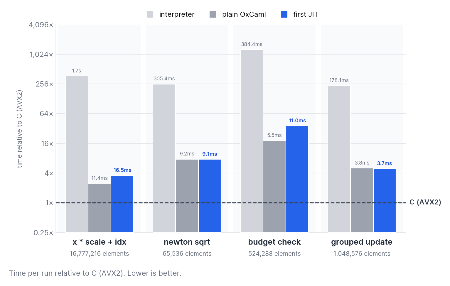
The benchmarks found that the JIT was much faster than the interpreter. However, the JIT was about the same speed (or slightly slower) than the manual OxCaml code and significantly slower than the C implementations. This wasn’t that surprising, since we hadn’t implemented any real optimizations or tuning in the compiler. Naturally, this needed to change if we wanted to catch up to the C implementations.

Optimizing using an intermediate representation

Sai then started looking at adding optimizations to the compiler. With the current compilation pipeline, this would have been slightly painful. Our front end representation was not designed to be easily analyzed or optimized. While that wouldn’t have necessarily stopped us from doing analysis, it’s often a better idea to add an intermediate representation (IR) that is more amenable to optimization. Sai implemented an IR based on A-normal form (ANF), a format where each intermediate value gets its own variable. This is the IR that we saw in the previous section about optimizing away control flow:

let%expect_test "IR: euclidean" =
  let lowered = For_testing.Ir.of_kernel (measure ~metric:Euclidean) in
  print_string (For_testing.Ir_body.to_string lowered.body);
  [%expect
    {|
    let n = shape[0]
    for i in n (normal) {
      let v = load_f32 in0[i]
      let v1 = load_f32 in1[i]
      let v2 = f32_sub v v1
      let v3 = f32_mul v2 v2
      store out[i] = v3
    }
    |}]
;;

let%expect_test "IR: manhattan" =
  let lowered = For_testing.Ir.of_kernel (measure ~metric:Manhattan) in
  print_string (For_testing.Ir_body.to_string lowered.body);
  [%expect
    {|
    let n = shape[0]
    for i in n (normal) {
      let v = load_f32 in0[i]
      let v1 = load_f32 in1[i]
      let v2 = f32_sub v v1
      let v3 = f32 0.
      let v4 = f32_ge v2 v3
      let v5 = f32_sub v3 v2
      let v6 = select v4 v2 v5
      store out[i] = v6
    }
    |}]
;;

The IR is more verbose but easier to analyze. For example, because all intermediate values are assigned a variable, it becomes easy to remove dead code; just look if an intermediate value is used anywhere after its definition.

Designing the IR to make code generation trivial

Sai designed this IR with a key design principle in mind: Generating the final OxCaml code from the IR should be a trivial process. Any interesting compilation logic should end up explicitly represented in the IR.

One instance of this principle shows up in how we model loops. As we mentioned before, kernels only declare what we do on each loop iteration, not how we loop over the code itself.

(fun graph [ x; scale ] [ Dim i ] -> exclave_
   let open (val Spmd.open_ graph) in
   let i = index i in
   F32.((x.!(i) *. broadcast scale.!(I32.lit #0l)) +. of_i32 i))

But in the IR, we explicitly specify the loop, as well as load/store logic. That way, the optimizer can reason about how to re-order or unroll loops. For example, the above kernel would produce the following IR:

let n = shape[0]
for i in n (normal) {
  let v = load_f32 in0[i]
  let v1 = i32 0
  let v2 = load_f32 in1[v1]
  let v3 = f32_mul v v2
  let v4 = f32_of_i32 i
  let v5 = f32_add v3 v4
  store out[i] = v5
}

The optimizer can analyze this IR and see that v1 and v2 do not depend on i and therefore can be lifted out of the loop:

let n = shape[0]
let v1 = i32 0
let v2 = load_f32 in1[v1]
for i in n (normal) {
  let v = load_f32 in0[i]
  let v3 = f32_mul v v2
  let v4 = f32_of_i32 i
  let v5 = f32_add v3 v4
  store out[i] = v5
}

It can also rewrite the loop to process 4 elements at a time, which reduces the amount of branching in the code.

let n = shape[0]
let v1 = i32 0
let v2 = load_f32 in1[v1]
for io in div n 4 (normal) {
  let i_0 = add (mul io 4) 0
  let i_1 = add (mul io 4) 1
  let i_2 = add (mul io 4) 2
  let i_3 = add (mul io 4) 3
  let v_0 = load_f32 in0[i_0]
  let v_1 = load_f32 in0[i_1]
  let v_2 = load_f32 in0[i_2]
  let v_3 = load_f32 in0[i_3]
  let v3_0 = f32_mul v_0 v2
  let v3_1 = f32_mul v_1 v2
  let v3_2 = f32_mul v_2 v2
  let v3_3 = f32_mul v_3 v2
  let v4_0 = f32_of_i32 i_0
  let v4_1 = f32_of_i32 i_1
  let v4_2 = f32_of_i32 i_2
  let v4_3 = f32_of_i32 i_3
  let v5_0 = f32_add v3_0 v4_0
  let v5_1 = f32_add v3_1 v4_1
  let v5_2 = f32_add v3_2 v4_2
  let v5_3 = f32_add v3_3 v4_3
  store out[i_0] = v5_0
  store out[i_1] = v5_1
  store out[i_2] = v5_2
  store out[i_3] = v5_3
}

By making the IR fairly explicit, we’re able to reason about—and therefore optimize—the code effectively.

Validating the IR backend

Like with the previous backend implementation, Sai put in a lot of work to validate the correctness of the new compilation path. He added the new backend to the existing cross-validation logic across the test suite, then added expect tests that printed the IR and the emitted OxCaml for various examples, which helped us confirm that the behavior was exactly as expected.

Once we were confident that the new IR-based path was correct, Sai deleted the previous backend.

How fast is the new backend?

With the current implementation, the IR backend generates essentially the same code as the first JIT, so the two perform about the same.

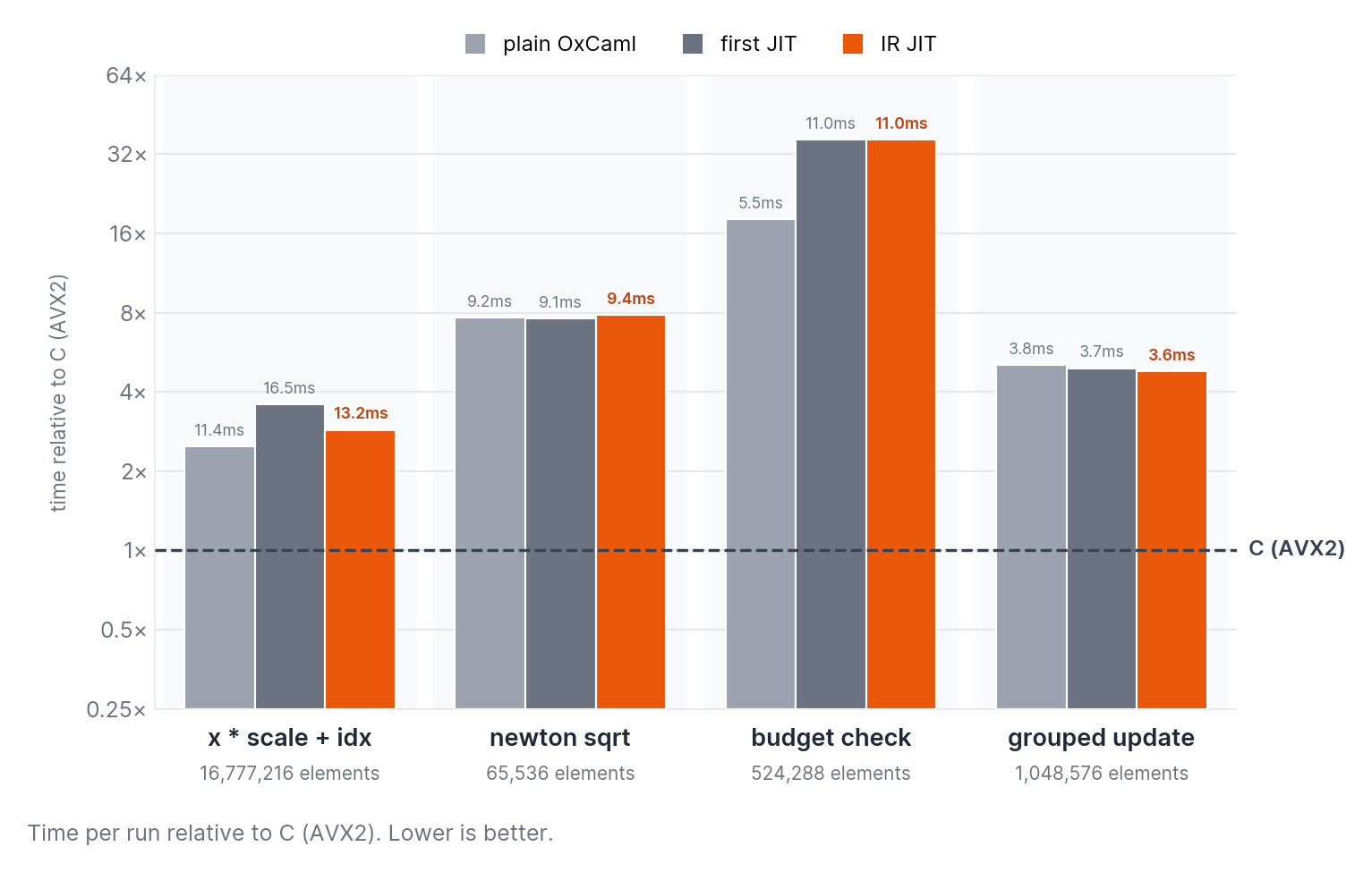
However, optimizations are now significantly easier to add. We’re currently working on adding vectorization and constant hoisting to the compiler. Preliminary benchmarks have found that these changes result in code that is on-par with our C AVX2 implementation.

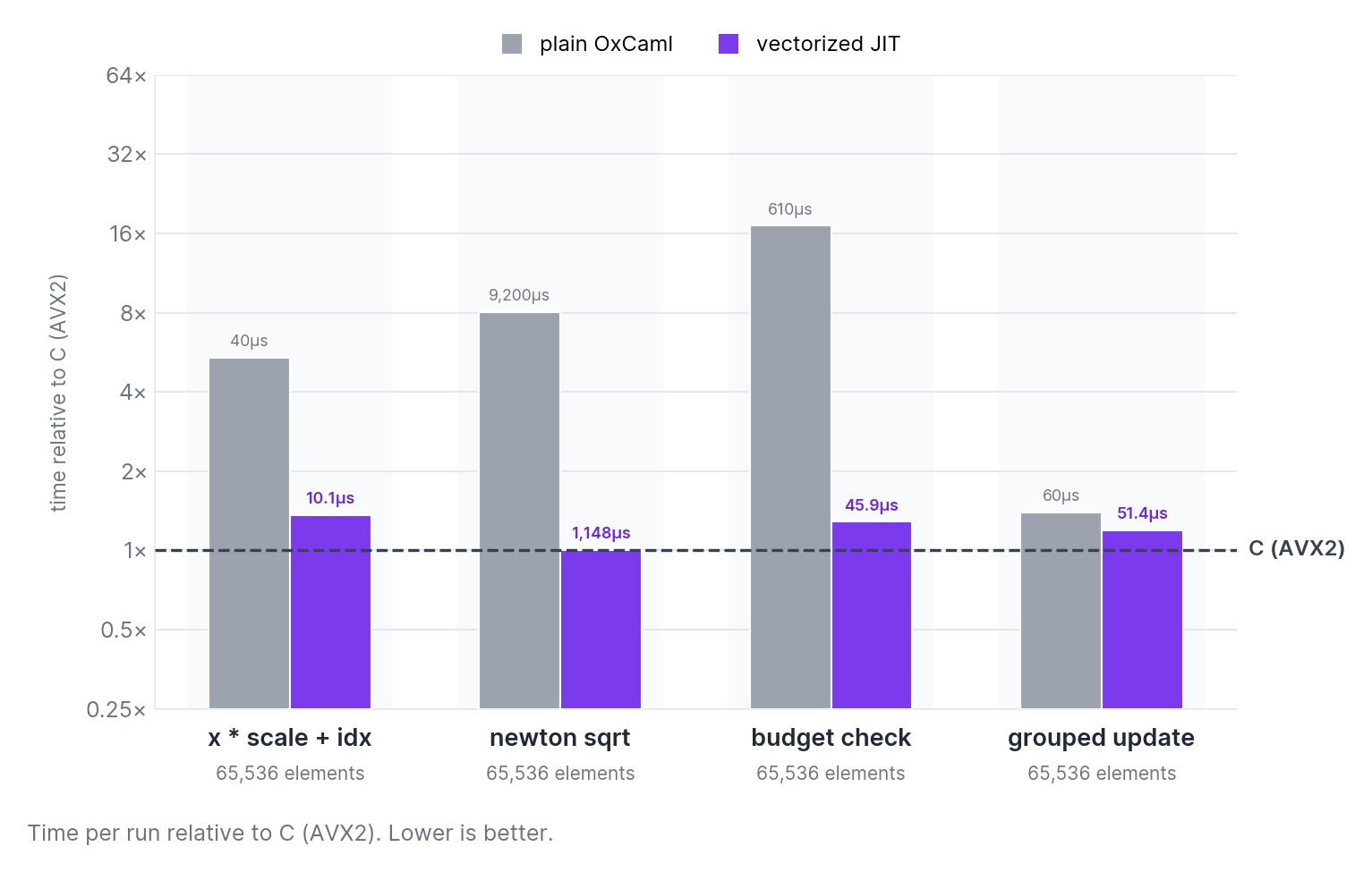
We’re also working on adding scheduling. Scheduling lets users customize how the kernel loops over the code with a sophisticated set of transformations like “split this loop into 8 piece chunks, vectorize these chunks, then unroll by 4”. Intelligent scheduling is important for getting the maximum possible performance out of the kernel. Eventually these schedules could also be auto-generated and benchmarked, so that the compiler can find the optimal one for your kernel.