The following is part of a series of posts about 2026 summer intern projects—for more, see “What the interns have wrought, special jumbo 2026 edition”

To compute gradients in the backward pass of model training, we need the activations (outputs) of computations. By default, PyTorch saves these activations during the forward pass so that they can be reused during the backward pass. Once we compute the gradients, we can free up the memory for the activations, producing the typical memory profile seen above, with a peak at the end of the forward pass and a trough at the end of the backward pass.

“Activation checkpointing” trades off some of this memory for compute. Instead of keeping an activation alive across the boundary, we discard it after we’ve used it in the forward pass; when we need it again to compute gradients in the backward pass, we just re-run the computation that produced it. Doing this en masse would be a bad idea, since you’d end up just repeating the entire forward pass during the backward pass. But if you could avoid storing some well-chosen nodes, you might find a better spot on the compute vs. memory frontier. (The fact that this is called “checkpointing” is confusing, because in fact the whole point is that we’re not saving the activation, but rather marking it as needing to be recomputed later.)

For his project this summer, Arsh Koneru, a software engineering intern on our ML Infra team, was tasked with building a better activation checkpointing scheme. Given a model spec and a memory budget, he’d have to find a set of nodes to drop that would minimize extra compute time while staying within the budget.

Why not just use…?

Arsh’s first task was to understand existing tools for activation checkpointing already built into PyTorch. In particular, when you call torch.compile, one of the phases is called AOT (Ahead-of-Time) Autograd. This computes a backward pass of your model in order to optimize over a joint graph both the forward and the backward. If there were no activation checkpointing, every activation generated by the forward pass would survive in the joint graph if it was directly needed by the backward pass. In the following computation, nodes a and b are saved from the forward pass but the backward pass needs b and c (since they are inputs into the orange nodes, u and v). So, in the backward pass, we also recompute c.

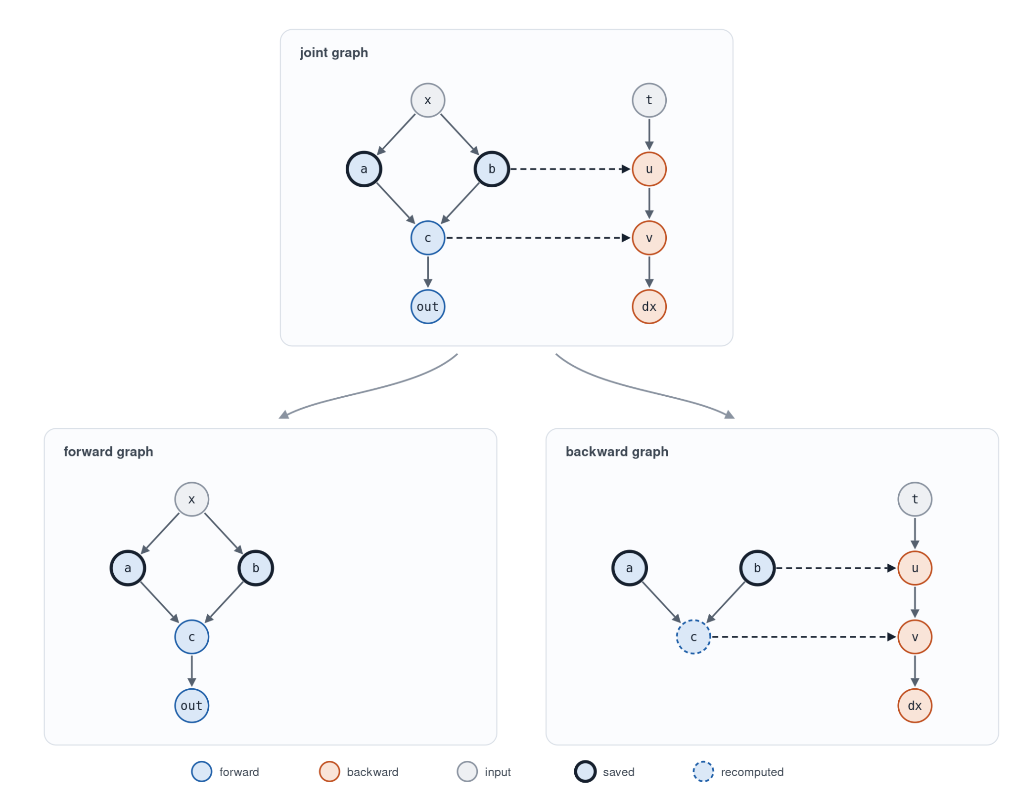
By default when you run your model in eager mode, nothing needed for the backward pass is ever dropped from the save set (so we would’ve saved b and c in the diagram above). But torch.compile applies an optimization. It drops some nodes from the save set using the min-cut partitioner, which improves runtime while also reducing memory. That may seem impossible, since we just said that activation checkpointing is a tradeoff between those two things; but there is a trick here. When Inductor, torch.compile’s default backend, generates kernels for a graph, it fuses cheap ops together. And sometimes it is actually faster to recompute a forward op and fuse it into a backwards kernel than it is to store the forward op output in memory and load it into our kernel, because of the cost of transferring data into and out of memory.

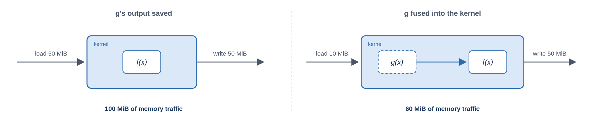
Note in the figure that if both ops g(x) (from the forward pass) and f(x) (from the backward pass) are memory-bound, then the fused kernel is actually faster, given the stipulated memory traffic.

So at a base level, PyTorch uses this min-cut optimization (with some restrictions and heuristics) to cut some nodes from the save set, namely those that are cheap and fusible.

But it also has another activation checkpointing mechanism given by the memory budget API. What this does is relax the min-cut rules in stages to propose more nodes to cut from the save set, solving a version of the knapsack problem to choose which ones.

This sounds like exactly the thing that Arsh was tasked with building, but in reality there were some major caveats with it:

• We didn’t love the API. You have to specify the budget as a percentage of the default torch compile activations to save, which is hard for users to reason about. We want to be able to specify an absolute actual total GB memory budget.
• It’s not monotonic: decreasing the budget from 20% to 10% can actually increase your peak memory usage (from extra memory used during the recomputation of the un-saved nodes).
• It doesn’t actually account for the true memory peak, or the true amount of time taken to recompute a node.

So Arsh set out to build an alternative with all the features we wanted.

How to compute the true memory and recomputation cost of a node

PyTorch actually also provides Selective Activation Checkpointing (SAC), which hands you each op in the graph and lets you decide whether to save or recompute it. But the full graph structure is invisible through this API: you only get to see one op at a time. This turns out not to be good enough.

To find the best ops to checkpoint, we need to see the entire graph, both to compute the true memory usage and the true recompute cost of each node.

Memory

We expect activation checkpointing to affect our memory usage like so:

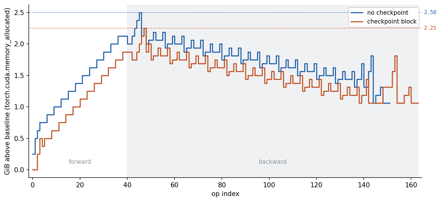
I.e., by eliminating a node from our save set in the forward pass, we expect the amount of memory not to climb as high during the forward pass, and therefore our peak should be lower.

However, it actually costs memory to recompute nodes in our graph. So if we recompute too aggressively or in the wrong places, we can end up with a higher peak. For instance, if we need to allocate many or large intermediate tensors during our recomputation, our peak can move to the recompute itself, and we get something looking like this:

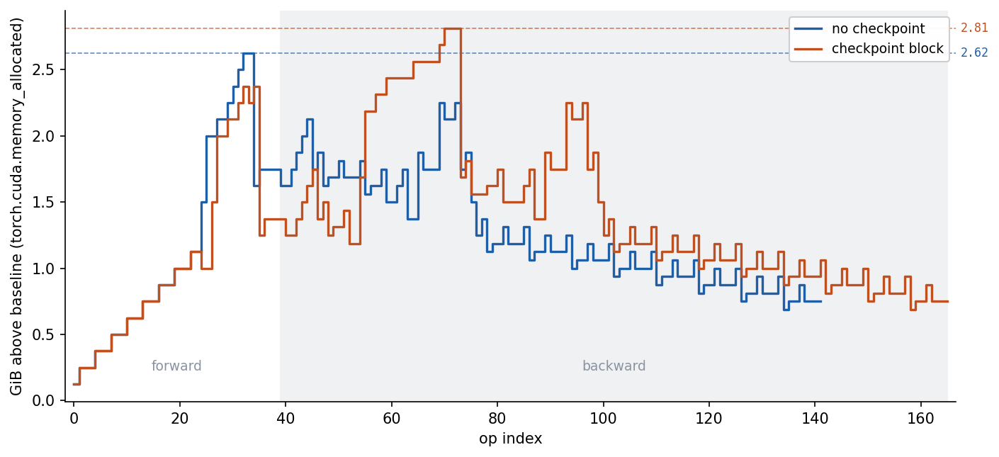
The checkpointing in this case both increases our peak memory and makes our training slower. Womp.

Recompute cost

Likewise, the cost of recomputing a node is actually the cost of recomputing everything needed to produce that node (or rather, everything that the backward pass would otherwise not have needed). In the below example, nodes a and b originally do not need to be computed in the backward pass, since their values are only used to produce c, which is saved.

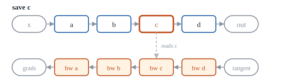
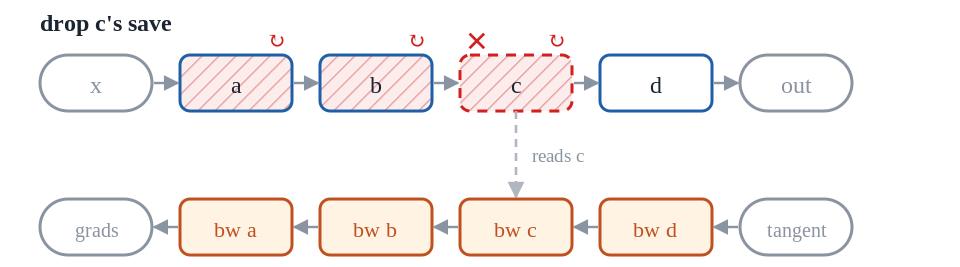
If we then choose to checkpoint c, i.e., to not save it, then we must now recompute a and b in our backward pass as well. This makes the cost of not saving c equal to a + b + c.

The new activation checkpointing procedure

Because it needs to see the whole graph, Arsh’s algorithm for activation checkpointing requires an extra pass compiling the model. This “planning” pass is run once, cheaply, on a single GPU before training.

The planning pass compiles the model on fake tensors, which carry shapes and dtypes but no data, and captures every graph it produces, plus the min-cut save set for each. (The min-cut is already a good activation checkpointing baseline since it usually reduces both memory and runtime. Starting there also reduces the search space, because nodes are fused, which makes planning faster.) While the graphs run, the planner also captures their execution order, e.g. A.fwd, B.fwd, B.bwd, A.bwd, as those will come in handy later.

Then, given the graphs and their save sets, the planner searches for a subset of min-cut saves to remove. (This new planner always does the same number or fewer saves, or rather frees more memory, than the min-cut baseline.) In particular, it greedily drops the save with the cheapest recompute cost per byte of peak memory freed. While the estimated peak is over the limit, for every output in the save set that can be dropped, the planner:

1. Derives the new forward and backward graphs from the new save set
2. Estimates the recompute cost of those new forward and backward graphs
3. Simulates by how many bytes removing this save would reduce the global memory peak
4. Removes the save having the best ratio, repeating until the limit is reached or no removal lowers the peak

A greedy algorithm isn’t optimal and can get stuck in a local minimum. (Dropping one save could change every other candidate’s cost, and the algorithm won’t discover that because it never backtracks.) Something like beam search might be better, but this was a good start.

To estimate peak memory, the planner then traverses both the forward and backward graphs and tracks which activations are alive at every step. Inputs are alive for the whole graph, and outputs are alive from their creation until the end of the graph. Any intermediate transient memory is kept alive until its last use within the graph. Meanwhile, parameters, buffers, and optimizer state stay allocated for the whole run, so those are measured separately (also on fake tensors), along with a user-provided reserve for what the planner can’t see: fragmentation, NCCL buffers, CUDA overheads, etc.

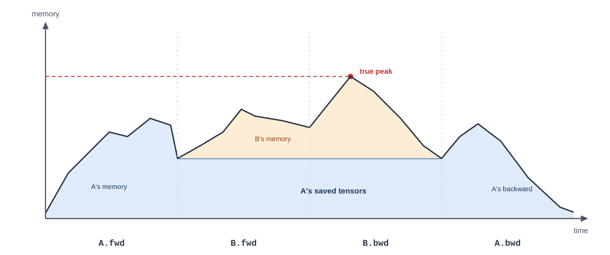
When there are multiple graphs stacked on top of each other, a tensor saved by graph A stays alive until A’s backward pass. Thus the true peak is the peak of that graph, plus everything the previous forward-pass graphs still have saved:

To estimate recompute time, the planner takes advantage of PyTorch’s formulas that produce the number of flops an operation takes given some input shape. (This is used by torch’s own knapsack algorithm.) The planner also treats the total flops of a graph as a proxy for how long it will take to recompute. In reality, not all flops are equal—it can depend on the datatype, on whether you’re using tensor cores, etc.—and not all compute-bound ops have a formula; and this completely ignores the time taken by memory-bound kernels. Finally, we adjusted for some common ops in our models that are much slower than their flop formulas would suggest. After all this, the planner’s approximation ended up being good enough for now.

Results

At training time, the plan is loaded and the joint graph is intercepted with a custom_partitioner. (Recall that the partitioner’s job is to take a joint graph and return the split forward and backward graphs.) Then, nodes are marked with MUST_SAVE and MUST_RECOMPUTE, min-cut is run again with these restriction tags, and that splits the graph into forward and backward passes that match what was planned.

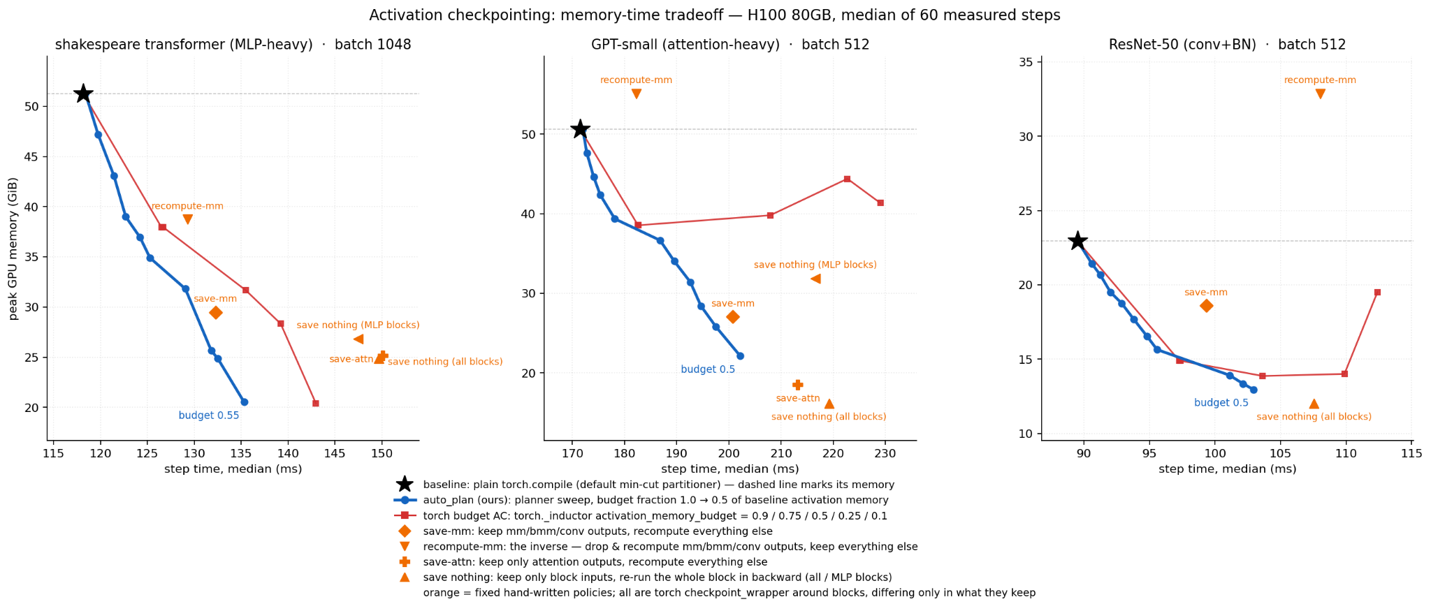
On the limited set of single-graph models that Arsh tested, auto-activation checkpointing (blue) beat the torch knapsack (red) and the op-level policies (orange) for most memory budgets. Points closer to the bottom-left of the graph indicate a faster activation checkpointing scheme for a given amount of peak memory.

Looking at memory profiles shows that activation checkpointing moves the peak memory to the recomputation in the backward pass. And you can also see one of the advantages of planning against the full graph: no single recomputation spike dominates peak memory. Instead, the memory profile is smoothed out across time, which makes sense as a strategy for staying under a threshold.

There are lots of improvements still to be made—the algorithm can be optimized; it doesn’t work on dynamic shapes or data-dependent ops (like torch.nonzero), and we can’t recompute ops that have an RNG state; various memory estimates are crude approximations; etc.—but Arsh’s work during the internship gives a promising baseline.

Looking forward to next summer…

If you’re interested in doing work like this, consider applying! You can find more details here: Jane Street Internships. Applications for our 2027 internship are now open!