
One of the problems we wrestle with at Jane Street is how to understand and manage the costs associated with the positions we hold: things like margin, financing costs, market risk, regulatory capital requirements, and so on. To that end, we’ve built systems that estimate these costs and propose ways to reduce them. Essentially, this is a numerical optimization problem.
This post describes a library we’ve developed to make that task
easier, called Gradient_calculator. With this library in hand,
we can write a computation just once, and get the ability to:
- Evaluate the computation to get its value
- Differentiate the computation with respect to all its variables automatically
- Debug it by inspecting intermediate values up to arbitrary levels of granularity
- Document it by auto-generating a LaTeX formula from the definition
And all of this functionality is provided while allowing programmers to express their computations in a natural style.
It’s worth saying that the core technique that powers
Gradient_calculator – automatic differentiation – is
by no means novel and in fact goes all the way back to Fortran in the
mid-60s. This post by Jane Street’s Max Slater explores
the wider field of differentiable programming in more detail. The
technique has become increasingly popular in the last decade or so,
especially in the context of training neural nets.
So lots of libraries that do this sort of thing already exist. Why did we build our own?
We ruled out some great open-source toolkits like JAX simply because they’re not easily interoperable with OCaml, which is what most of our production systems are written in. But even frameworks with OCaml bindings, like OWL and ocaml-torch, tended to model computations abstractly as operations over vectors and matrices (or, more generally, tensors), which did not seem like the most natural way to read, write, or think about the computations we typically want to model ourselves. Our computations also aren’t as black-box-y as a neural net; often there’s a well-defined equation that describes them.
By developing our own library specifically for these kinds of computations, we could really focus on making it work well in our context.
What’s more, we had greater control over its design and functionality, and capitalized on that by adding support for debugging and documenting computations, features we didn’t find in existing solutions.
A toy example
Let’s demonstrate how this all works with a toy example, using the
Computation module exposed by the Gradient_calculator
library. Suppose we have the following equation:
where initially and . Expressed as a computation,
it looks like:
open! Computation

let computation =
  let var name initial_value =
    variable (Variable.create ~id:(Variable.ID.of_string name) ~initial_value)
  in
  let x = var "x" 2. in
  let y = var "y" 4. in
  square (sum [x; square (sum [ y; constant 1.0 ])])
;;
If we do the math by hand, we would find that the partial derivatives of this are:
And indeed, we can confirm that Computation knows how to compute this
too, with a simple expect test.
let%expect_test _ =
  Computation.For_testing.print_derivatives computation;
  [%expect
    {|
    ┌──────────┬─────────┐
    │ variable │   ∂f/∂v │
    ├──────────┼─────────┤
    │        x │  54.000 │
    │        y │ 540.000 │
    └──────────┴─────────┘ |}]
;;
The library API, simplified
Here is a simplified, stripped-down version of the Computation
module:
open! Core

(** A computation involving some set of variables. It can be evaluated, and
    the partial derivative of each variable will be automatically computed. *)
type t

module Variable : sig
  (** An identifier used to name a variable. *)
  module ID : String_id.S

  (** A variable in a computation. *)
  type t

  val create : id:ID.t -> initial_value:float -> t

  (** Returns the current value of this variable. *)
  val get_value : t -> float

  (** Returns the current partial derivative of this variable. *)
  val get_derivative : t -> float

  (** Sets the current value of this variable. *)
  val set_value : t -> float -> unit
end

(** Constructs a computation representing a constant value. *)
val constant : float -> t

(** Constructs a computation representing a single variable. *)
val variable : Variable.t -> t

(** Constructs a computation representing the sum over some [t]s. *)
val sum : t list -> t

(** Constructs a computation representing the square of [t]. *)
val square : t -> t

(** [evaluate t] evaluates the computation [t] and returns the result, and
    updates the derivative information in the variables in [t]. *)
val evaluate : t -> float
The key points to take away here are:
-
Computation.ts can be constructed directly, for example viaconstantandvariable, or by composing existingComputation.ts (e.g. viasumandsquare). -
We store information about the values and partial derivatives of each variable, and the latter is updated whenever the computation is evaluated.
This API hides the internal details related to computing derivatives,
and packages everything up in a uniform way: values of type
Computation.t. This lets us easily build on top of this
abstraction. For example, we can write a gradient descent algorithm
that operates on any given Computation.t: all we need is the
ability to evaluate it and extract information about its partial
derivatives at each step, which every Computation.t allows us to
do.
The library also provides a special function that lets one specify a
black-box calculation in which the cost and partial derivatives are
computed “by hand”, likewise packaging the result up as a
Computation.t. This is useful when the base primitives are
insufficient, or when the computation has already been implemented
elsewhere.
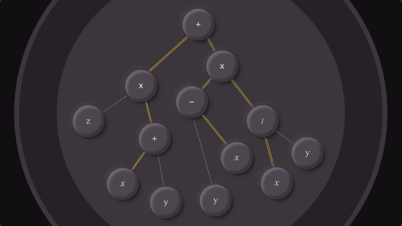
A peek under the hood
As described earlier, internally, a Computation.t is represented
as an expression tree, where each node is either a leaf representing
some terminal value (like a constant or a variable) or an internal
node performing some operation over other nodes (e.g. a summation or
square).
Upon constructing a Computation.t, no evaluation is actually
performed. It’s only when evaluate is called that we do any
work. In particular, we’ve implemented forward-mode AD, in which we
are performing the evaluation of our function and computing the
partial derivatives at the same time, in a single “forward” pass. The
cost is approximately proportional to the cost of evaluating the
function itself, since we’re mostly just doing some constant
additional work for each operation. This is much better than numerical
differentiation.
For operations involving frequent, nested applications of the chain rule, reverse-mode AD can be even more efficient than forward-mode AD. However, implementations of reverse-mode AD require tracking more intermediate state and are generally more complicated. Given the computations we were modeling involve few nested applications of the chain rule, the performance benefits of reverse-mode AD did not outweigh its complexity costs.
Real-world example: calculating the net market value of our positions
Let’s try this out with an example that is more representative of computations we typically write in real systems. Suppose we want to compute the absolute net market value of our positions, with positions netted within our accounts at each bank. First, let’s mock out our positions and some market prices.
let positions : float Ticker.Map.t Account.Map.t Bank.Map.t =
  [ "AAPL", "BANK A", "ACCOUNT W", 10
  ; "AAPL", "BANK B", "ACCOUNT X", -20
  ; "AAPL", "BANK A", "ACCOUNT Y", 20
  ; "AAPL", "BANK B", "ACCOUNT Z", 10
  ; "GOOG", "BANK A", "ACCOUNT W", -5
  ; "GOOG", "BANK B", "ACCOUNT X", 30
  ; "GOOG", "BANK A", "ACCOUNT Y", 15
  ; "GOOG", "BANK B", "ACCOUNT Z", -30
  ]
  |> List.map ~f:(fun (ticker, bank, account, quantity) ->
    Bank.of_string bank, (Account.of_string account, (Ticker.of_string symbol, Int.to_float quantity)))
  |> Map.of_alist_multi (module Bank)
  |> Map.map ~f:(Map.of_alist_multi (module Account))
  |> Map.map ~f:(Map.map ~f:(Map.of_alist_multi (module Ticker)))
  |> Map.map ~f:(Map.map ~f:(Map.map ~f:(List.sum (module Float) ~f:Fn.id)))
;;

let prices : float Ticker.Map.t =
  [ "AAPL", 10; "GOOG", 15 ]
  |> List.map ~f:(fun (ticker, price) -> Ticker.of_string ticker, Int.to_float price)
  |> Map.of_alist_exn (module Ticker)
;;
Here’s how you might write the (eager) computation normally:
let%expect_test _ =
  let cost_for_one_position (ticker, quantity) =
    let price = Map.find_exn prices ticker in
    quantity *. price
  in
  let cost_for_one_account by_ticker =
    Float.abs (List.sum (module Float) (Map.to_alist by_ticker) ~f:cost_for_one_position)
  in
  let cost_for_one_bank by_account =
    List.sum
      (module Float)
      (Map.data by_account)
      ~f:cost_for_one_account
  in
  let cost = List.sum (module Float) (Map.data positions) ~f:cost_for_one_bank in
  print_endline (Float.to_string_hum cost);
  [%expect {| 1_050.000 |}]
;;
This is pretty standard stuff. However, this calculation is difficult
to incorporate into an optimization like gradient descent since we
don’t have any information about derivatives. Here’s how you’d convert
the same calculation to use the Computation API:
!  let cost_for_one_position bank account (ticker, quantity) =
     let price = Map.find_exn prices ticker in
+    Computation.variable
+      (Computation.Variable.create
+         ~id:
+           (Computation.Variable.ID.of_string
+              (sprintf !"%{Ticker} @ %{Bank}/%{Account}" ticker bank account))
!         ~initial_value:(quantity *. price))
   in
!  let cost_for_one_account bank (account, by_ticker) =
-    Float.abs (List.sum (module Float) (Map.to_alist by_ticker) ~f:cost_for_one_position)
!    Computation.abs
!      (Computation.sum
!         (List.map (Map.to_alist by_ticker) ~f:(cost_for_one_position bank account)))
   in
!  let cost_for_one_bank (bank, by_account) =
-    List.sum (module Float) (Map.data by_account) ~f:cost_for_one_account
!    Computation.sum (List.map (Map.to_alist by_account) ~f:(cost_for_one_account bank))
   in
-  let cost = List.sum (module Float) (Map.data positions) ~f:cost_for_one_bank in
!  let cost = Computation.sum (List.map (Map.to_alist positions) ~f:cost_for_one_bank) in
!  print_endline (Float.to_string_hum (Computation.evaluate cost));
   [%expect {| 1_050.000 |}]
As you can see, the code looks pretty similar: we’re mostly swapping
out List.sum for Computation.sum, Float.abs for
Computation.abs, and declaring our
Computation.Variable.ts. The result of evaluating it is the
same, which is obviously good. Further, we now have the partial
derivatives for each of our variables:
let%expect_test _ =
  (* same as above *)
  Computation.For_testing.print_derivatives cost;
  [%expect
    {|
    ┌─────────────────────────┬────────┐
    │                variable │  ∂f/∂v │
    ├─────────────────────────┼────────┤
    │ AAPL @ BANK A/ACCOUNT W │  1.000 │
    │ AAPL @ BANK A/ACCOUNT Y │  1.000 │
    │ AAPL @ BANK B/ACCOUNT X │  1.000 │
    │ AAPL @ BANK B/ACCOUNT Z │ -1.000 │
    │ GOOG @ BANK A/ACCOUNT W │  1.000 │
    │ GOOG @ BANK A/ACCOUNT Y │  1.000 │
    │ GOOG @ BANK B/ACCOUNT X │  1.000 │
    │ GOOG @ BANK B/ACCOUNT Z │ -1.000 │
    └─────────────────────────┴────────┘ |}]
;;
Intuitively, these results makes sense. We’re net “long” in every bank
account except BANK B/ACCOUNT Z, so an extra dollar there
reduces our absolute net market value and therefore our overall cost, whereas an
extra dollar anywhere else increases it.
Debugging computations
We don’t have to stop here. By virtue of our representation of computations as statically defined trees, we can do some pretty powerful things.
In particular, as we’re evaluating a computation, we’re traversing the entire tree and evaluating the value at each node. We can track that information as we go and display it in an expect-test-friendly way:
let%expect_test _ =
  (* same as above *)
  Computation.For_testing.print_debug_tree cost;
  [%expect
    {|
    ◉ SUM(...): 1050.00
    ├──◉ SUM(...): 450.00
    |  ├──◉ ABS(...): 25.00
    |  |  └──◉ SUM(...): 25.00
    |  |     ├──• AAPL @ BANK A/ACCOUNT W: 100.00
    |  |     └──• GOOG @ BANK A/ACCOUNT W: -75.00
    |  └──◉ ABS(...): 425.00
    |     └──◉ SUM(...): 425.00
    |        ├──• AAPL @ BANK A/ACCOUNT Y: 200.00
    |        └──• GOOG @ BANK A/ACCOUNT Y: 225.00
    └──◉ SUM(...): 600.00
       ├──◉ ABS(...): 250.00
       |  └──◉ SUM(...): 250.00
       |     ├──• AAPL @ BANK B/ACCOUNT X: -200.00
       |     └──• GOOG @ BANK B/ACCOUNT X: 450.00
       └──◉ ABS(...): 350.00
          └──◉ SUM(...): -350.00
             ├──• AAPL @ BANK B/ACCOUNT Z: 100.00
             └──• GOOG @ BANK B/ACCOUNT Z: -450.00 |}]
;;
We’ve found this to be quite useful in practice. For one thing, it makes debugging a lot easier. Instead of littering our code with print statements we can inspect all intermediate values at once.
The expect-test integration encourages an exploratory style, in which we begin with some small part of the computation and incrementally build on it until the entire function is complete. This has proved useful when writing computations from scratch, when the incidence of bugs tends to be the highest.
Further, because we’re observing more than just the final value, we
can be more confident that the final calculation is correct. For
example, suppose we have a function consisting of a series of nested
max operations. For any given set of inputs, we’re only
exercising some subset of the paths in the calculation, and the final
value only reflects a subset of terms. It may be that the terms on
some unexercised paths are actually calculated incorrectly; by
printing out all intermediate values, this becomes much harder to
miss.
Finally, these expect-tests make it easier to understand and review logical changes in the calculation, regardless of what’s changed in the code.
Note that it’s possible to avoid printing out an unreadably large tree for complex calculations by limiting the depth to which the tree is printed and/or by only including particularly tricky terms.
Documenting computations
Time for one more magic trick. As with any calculation, once you’ve implemented it, you should take the time to document it. We do this a lot, but manual documentation inevitably grows stale, and eventually fallow, and it may no longer reflect the actual implementation. Luckily, since we know their structure, we can automatically generate documentation for our computations. Let’s try this out:
let%expect_test _ =
  (* same as above *)
  cost |> Computation.to_LaTeX_string |> print_endline;
  [%expect
    {|
    \left(\left| \left(\texttt{AAPL @ BANK A/ACCOUNT W} + \texttt{GOOG @ BANK A/ACCOUNT W}\right) \right| + \left| \left(\texttt{AAPL @ BANK A/ACCOUNT Y} + \texttt{GOOG @ BANK A/ACCOUNT Y}\right) \right|\right) + \left(\left| \left(\texttt{AAPL @ BANK B/ACCOUNT X} + \texttt{GOOG @ BANK B/ACCOUNT X}\right) \right| + \left| \left(\texttt{AAPL @ BANK B/ACCOUNT Z} + \texttt{GOOG @ BANK B/ACCOUNT Z}\right) \right|\right) |}]
;;
Now let’s render that in a LaTeX block:
That’s technically correct, but not all that useful. It’s documenting the specific computation we’re evaluating, not its generalized form. We can resolve this by introducing some “metavariables”. In essence, a metavariable is a symbol that’s used in a formula – it doesn’t represent an actual variable in the computation. Annotating a given computation to use metavariables is straightforward. In the example above, we can write:
     let price = Map.find_exn prices ticker in
-    Computation.variable
+    Computation.variablei
+      ~to_LaTeX:(fun [ (`ticker, ticker); (`account, account); (`bank, bank) ] ->
+        "MktVal"
+        |> Nonempty_string.of_string_exn
+        |> LaTeX.of_alpha_exn
+        |> LaTeX.mathsf
+        |> LaTeX.function_application
+             ~args:
+               [ LaTeX.of_metavariable ticker
+               ; LaTeX.of_metavariable bank
+               ; LaTeX.of_metavariable account
+               ])
       (Computation.Variable.create
          ~id:
            (Computation.Variable.ID.of_string
               (sprintf !"%{Ticker} @ %{Bank}/%{Account}" ticker bank account))
          ~initial_value:(quantity *. price))
   in
   let cost_for_one_account bank (account, by_ticker) =
     Computation.abs
-      (Computation.sum
+      (Computation.sumi
+         ~metavariable:Metavariable.(of_string "ticker" <~ `ticker)
          (List.map (Map.to_alist by_ticker) ~f:(cost_for_one_position bank account)))
   in
   let cost_for_one_bank (bank, by_account) =
-    Computation.sum (List.map (Map.to_alist by_account) ~f:(cost_for_one_account bank))
+    Computation.sumi
+      ~metavariable:Metavariable.(of_string "account" <~ `account)
+      (List.map (Map.to_alist by_account) ~f:(cost_for_one_account bank))
-  in
-  let cost = Computation.sum (List.map (Map.to_alist positions) ~f:cost_for_one_bank) in
+  in
+  let cost =
+    Computation.sumi
+      ~metavariable:Metavariable.(of_string "bank" <~ `bank)
+      (List.map (Map.to_alist positions) ~f:cost_for_one_bank)
+  in
Already this results in much more legible LaTeX output:
Now, suppose we need to modify our calculation to multiply the
absolute net market value at each bank by some predefined rate, which varies across
banks. As soon as we update the definition of our Computation.t
and attach the relevant documentation information to new terms, our
auto-generated LaTeX formula updates as expected:
Optimizing computations
As we mentioned at the beginning of the post, the motivating use-case
for developing Gradient_calculator was to provide developers a
way to easily construct computations that could be optimized using
gradient descent. The library provides an implementation of gradient
descent that builds on top of the Computation.t abstraction. In
particular, it exposes an optimize function which takes in some
Computation.t and determines the values to assign to variables
in order to minimize that computation. Let’s see this in action,
revisiting our toy example:
let%expect_test _ =
  let context = Evaluation_context.initialize computation in
  let%bind outcome =
    Gradient_descent.optimize ~debug:true computation context ~step_size:(Fixed 1e-2)
  in
  print_s ([%sexp_of: Gradient_descent.Outcome.t] outcome);
  [%expect {| (Converged (on_iter 1418)) |}];
  For_testing.print_debug_tree computation;
  [%expect
    {|
    ◉ SQUARE(...): 0.000
    └──◉ SUM(...): 0.000
       ├──• x: -0.000
       └──◉ SQUARE(...): 0.000
          └──◉ SUM(...): -0.021
             ├──• y: -1.021
             └──• CONST: 1.000 |}];
  return ()
;;
As we’d expect, and is a minimum of our function.
To our more realistic net market value example, we would do something
similar, except we’d want to pass additional constraints to
optimize to ensure that our overall position in each ticker
across all accounts remains the same. (After all, we’re looking for
the optimal set of transfers to make across accounts, but we aren’t
reducing or increasing the total number of shares we hold in each
ticker.)
Future work
There’s still a long list of things we can do to further improve this library. Here are just a few ideas our team is thinking about:
Support for incrementality
Every time evaluate is called, the entire tree is traversed and
values are recomputed from scratch. We could instead have
evaluate run incrementally, only recomputing the values and
derivatives for variables whose values changed and any other dependent
nodes (transitively).
Compiler-inspired optimizations
We can think of our Computation.t as a sort of “intermediate
representation” of a computation, with Gradient_calculator’s
constructors serving as the “front-end” (i.e. going from some
specification of a computation to a concrete Computation.t) and
the evaluate function serving as the “back-end” (i.e. going from
this Computation.t to a value plus derivative information plus a
LaTeX formula and so on…). Drawing inspiration from some common
compiler optimizations, we could add support for constant folding,
common sub-expression elimination, etc. so that our IR
Computation.t is simplified as much as possible. Some of these
optimizations may require us to represent our Computation.t as a
DAG as opposed to a tree.
Automatic differentiation using algebraic effects
Algebraic effects, landing in OCaml 5.0, could provide a mechanism for implementing automatic differentiation using effect handlers, as described in this paper and demonstrated in this GitHub example. This would obviate the need to represent computations as trees, which would present a more memory-efficient alternative at the expense of some of the other features discussed in this post.
Alternative display formats
Currently, we only support printing the debug tree as an ASCII diagram and the formula in LaTeX. We could add support for alternative display formats as well (e.g., an SVG version of the tree) so that this information can be rendered in the most suitable way.
Open-sourcing the project
Our plan is to release this project as an open source tool soon, at which point we’ll be eager for any other ideas, suggestions, or feedback.