

At Jane Street, we have some experience using FPGAs for low-latency systems–FPGAs are programmable hardware where you get the speed of an application-specific integrated circuit (ASIC) but without being committed to a design that’s burned into the chip. It wasn’t so long ago that FPGAs were expensive and rare, but these days, you can rent a $5,000 card on the Amazon AWS cloud for less than $3 an hour.
Recently, my entry in a competition for a decades-old puzzle showed how clever use of FPGAs can be used to push the boundaries of low-latency computing.
Cryptographic puzzles
Back in 1999, MIT’s Computer Science and Artificial Intelligence Lab created a time capsule that included a cryptographic puzzle designed by Ron Rivest (the “R” in RSA). The puzzle was to calculate 22t (mod n) for t = 79,685,186,856,218 and a 2048-bit semiprime modulus n. (A semiprime is the result of multiplying two primes together.) The prompt helpfully pointed out that the problem could be solved by starting from 2 and repeatedly squaring t times mod n. For example (from the prompt):
Suppose n = 11*23 = 253, and t = 10.  Then we can compute:
	2^(2^1) = 2^2 = 4 (mod 253)
	2^(2^2) = 4^2 = 16 (mod 253)
	2^(2^3) = 16^2 = 3 (mod 253)
	2^(2^4) = 3^2 = 9 (mod 253)
	2^(2^5) = 9^2 = 81 (mod 253)
	2^(2^6) = 81^2 = 236 (mod 253)
	2^(2^7) = 236^2 = 36 (mod 253)
	2^(2^8) = 36^2 = 31 (mod 253)
	2^(2^9) = 31^2 = 202 (mod 253)
	w = 2^(2^t) = 2^(2^10) = 202^2 = 71 (mod 253)
Rivest’s team chose the number of squarings t so that, if Moore’s Law held up, the puzzle would take around 35 years to crack.
We can expect internal chip speeds to increase by a factor of approximately 13 overall up to 2012, when the clock rates reach about 10GHz. After that improvements seem more difficult, but we estimate that another factor of five might be achievable by 2034. Thus, the overall rate of computation should go through approximately six doublings by 2034.
But then in 2019 it was announced that Belgian programmer Bernard Fabrot had been able to crack the puzzle in just three and a half years, a decade and a half ahead of schedule. There were no magic tricks in his approach. It was just that Rivest’s original estimate was off by a factor of ten. While we don’t have 10GHz CPUs sitting in our desktops (mainly due to thermal issues), CPU and multi-core architecture has advanced dramatically. A few weeks after Bernard announced that he solved the puzzle, another group called Cryptophage announced they had, too, using FPGAs in just two months.
An interesting aspect of this puzzle is that while it’s expensive to compute, it’s cheap for the designer of the puzzle to verify the solution. That’s because if you know the two primes p and q that are the factors of n, you can use Euler’s totient function to calculate phi(n) = (p-1)(q-1). Once you have that, the large exponent can be reduced from 22t (mod n) to a much faster to calculate 22t (mod phi(n)) (mod n).
These types of cryptographic puzzles are part of a class of Verifiable Delay Functions (VDF): problems that take some medium to large quantity of non-parallelizable work to compute, but that can be verified quickly. They are useful in decentralized blockchain systems, for instance for randomness beacons, voting, and proofs of replication. While Rivest’s puzzle required secret knowledge to quickly verify the result, there are many proposed constructions that allow a VDF to be publicly verified without secret knowledge.
Using FPGAs for low latency
In late 2019, the VDF alliance began a competition to find the lowest latency achievable for a VDF problem similar to Ron Rivest’s 1999 puzzle. The idea was that by submitting such problems to fierce competition, you could help battle-test systems that rely on VDFs.
The competition required participants to solve a scaled-down version of the Rivest puzzle, with a t of ~233 instead of 246, and a 1024-bit modulus. Contestants were also given p in advance.
Ozturk multiplier
The winner from the first round of the VDF alliance competition was Eric Pearson, using an Ozturk multiplier architecture. This type of multiplier takes advantage of a couple of tricks that FPGAs can do extremely efficiently that GPUs or CPUs can’t:
-
Redundant bit representation (RBR). This means your 1024-bit number is split into n equally-sized words (in this case n = 64 words, each 16 bits), but then each word gets an extra redundant bit. The advantage of this is when you accumulate all the partial products from a multiplication, you don’t need to propagate carry bits through the whole 2048-bit result–you only need to propagate it to the neighboring word. On an FPGA, the maximum speed your circuit can operate will be limited by the slowest path–which is often the carry chain. This helps makes the squaring part of the equation run as fast as possible. When we square, we use the same algorithm as multiplication, except half of the partial products are identical. We don’t need to calculate them twice: we just bit shift them by 1 bit, essentially doubling them for free.
-
Modulo reduction using lookup tables. Every bit that is set past the 1024-bit modulo boundary can be precalculated as a modulo p value and added back onto the original result–e.g., 22000 becomes 22000 % p. This way, a 2048-bit result can be reduced back to a 1024 + log2(height of the pre-computed word tree) bit modulo p value. This takes a lot of memory on the FPGA, but allows you to calculate modulo p in just three clock cycles: two to look up RAM, one to fold the offsets back into the result. Both this technique and using RBR help speed up the final “modulo p” step required by the VDF equation.
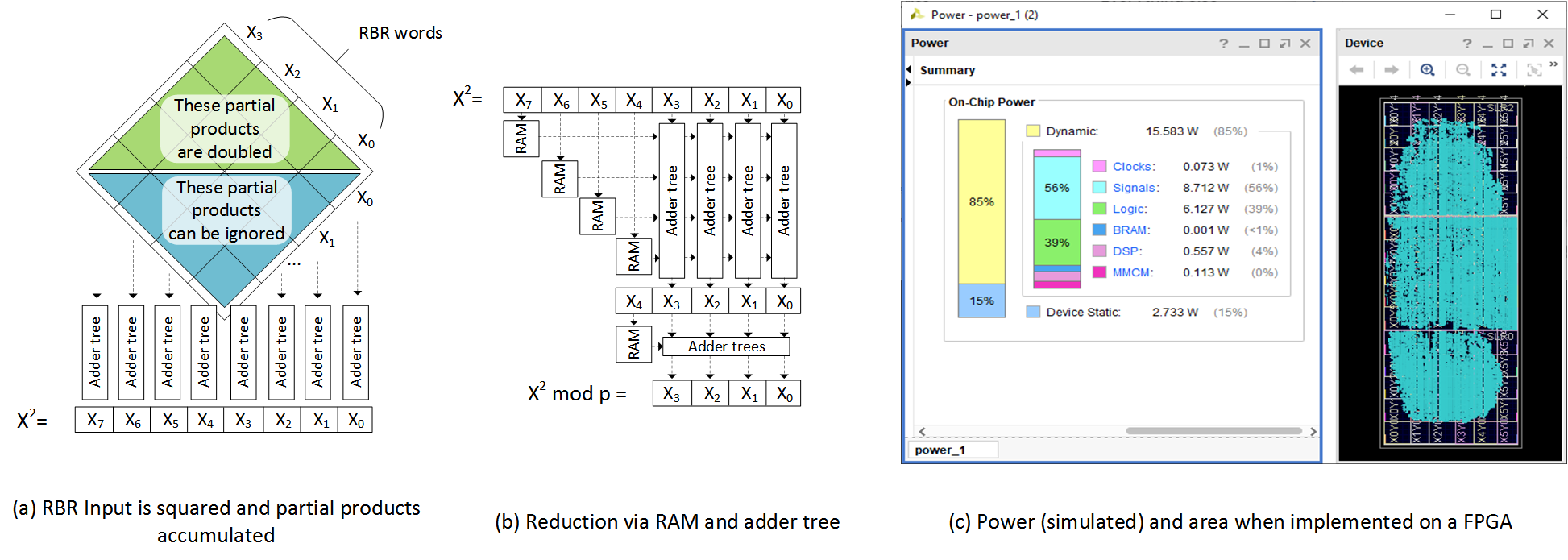
Eric’s implementation took advantage of the LUT size in this generation of FPGA (6 input) to more efficiently map the memory reduction elements and compression trees in the multiplier partial product accumulation. For the modulo reduction, instead of block RAMs he used the faster LUTRAM, which further saves a clock cycle; taking this saved clock cycle to add more pipelining to paths where timing was critical allowed for an operating frequency of 158.6MHz (total 4-stage pipeline). This meant a single iteration of the VDF could be performed in 25.2ns. The design spanned most of the FPGA, crossed multiple super logic regions (abbreviated SLR, these are individual silicon dies that are used to form one large chip), and required power management to run. Eric commented in his submission that the FPGA actually burns as much as 48W when running in the AWS cloud.
Predictive Montgomery multiplier
There was a third and final round of the competition where more alternative approaches to the problem were encouraged–the Ozturk multiplier code was actually supplied in a basic form for the first rounds, so it was important to make sure there wasn’t some alternative design that might be faster than Ozturk. (Initially, no one wanted to spend the time trying to implement something from scratch only to find out it was not as good.) This sounded interesting to me so I came up with a novel “Predictive Montgomery multiplier” architecture which was the final round winner.
Tricks I used (again not efficiently possible on GPUs or CPUs):
-
Montgomery multiplication with RBR. I decided to implement the modulo reduction scheme using Montgomery’s algorithm, which requires a transform into a Montgomery domain–but then modulo p becomes a fixed bit-shift which can be done on a FPGA in O(1) time. I only transform in and out of the Montgomery domain at the start and end of our 2n loops, so the overhead is not noticeable. I also modified the algorithm to work with RBR–this makes each individual step a little bit faster.
Montgomery multiplication only involves multiplications, additions, and bit shifts–all of which are easy to implement in RBR, and will benefit from the shorter carry-chain. I also add an extra RBR word so that in total there are 65 words each of 17 bits to represent a 1024-bit number. This change allows a modification to the Montgomery algorithm so that it is guaranteed to produce a result less than p (a traditional Montgomery algorithm only brings the result to less than 2p). By using Montgomery multiplication I was able to save on a lot of FPGA area because the modulo step of the VDF equation becomes much easier.
-
Log-3 compressor circuit with fast-carry. I decided to implement my multiplier as a simple cross-product multiplier using FPGA DSPs (digital signal processors, a small dedicated resource on the FPGA for performing multiplication efficiently). The chosen RBR bit width of 17 means one partial product only takes 1 DSP resource, followed by a final partial product accumulation stage using general FPGA LUTs. The maximum height of the tree used requires 128 columns, each containing 129 partial products, each 17 bits wide to be added together. I experimented with different log values and found folding the tree with arity 3, and using the FPGA adder fast-carry (rather than using compressor trees which did not utilize the fast-carry) gave the best results. This style of compressor implemented with RBR allowed me to squeeze even more performance out of the multiplier than before.
-
Predictive branching. Montgomery multiplication requires a full 1024-bit squaring, followed by a 1024-bit multiplication where I only care about the lower 1024 bits of the result, followed by a 1024-bit multiplication, addition, and bit shift down (so I essentially only care about the upper 1024 bits of the result).
The problem here is that a single SLR on the FPGA only has 2280 DSPs–and I really wanted to work in this budget, since communicating with multiple SLRs can make the whole design slower. A single squaring takes around 2120 DSPs, but a full multiplication will take 4225. To solve this problem I use predictive branching: the multiplier calculates partial products based on an inputs fed in via a crossbar, where the inputs are selected so I’m only calculating a full square, the lower 65 + x words, or the upper 65 + x words. Here x is the number of words past the boundary I calculate, to make sure I account for any carry overflow that might be getting erroneously included or discarded due to our RBR form.
If I detect in the boundary words that might have this case (detected by all 1s and no free bits to absorb carry), I will branch and calculate the full 2048-bit (130-word) result, with the carry fully propagated. This is so rare that it hardly impacts performance, but this style of predictive branching allows us to implement the entire Montgomery RBR algorithm using a single SLR and 2272 DSPs. I also take advantage of the partial product tree and shortcut the extra addition in there without adding extra pipeline stages.
-
Slower, shorter pipeline. Often, pipeline stages can be added to allow a design to achieve a higher frequency and higher throughput. But since this is for low latency, you actually don’t want to pipeline more than necessary–extra pipelines will increase the routing latency on signals in the FPGA as they now need to make “pit stops” to access the register. In my design, the main data path loop only has a single pipeline stage on the output of the predictive multiplier, which directly feeds back into the multiplier crossbar. This improvement not only helps improve latency, but also reduce the overall power used in the design. A slower clock means individual signals will be switching at a lower frequency, which leads to a quadratic reduction in power consumed on the FPGA.
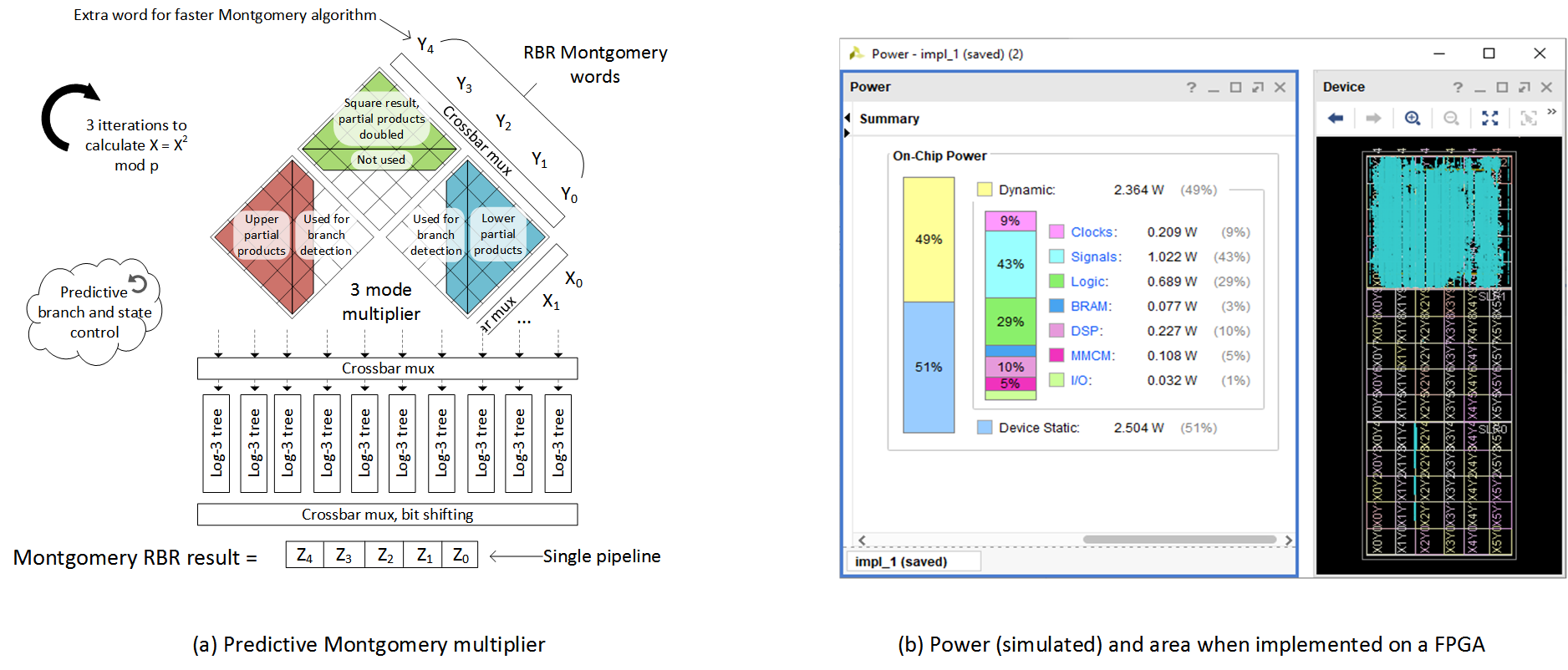
My multiplier design ran at 65MHz and took 46ns (3 clock cycles) to finish one iteration of the VDF. It could be fully implemented on one SLR of the FPGA (a third of the FPGA, 2.3x less than the Ozturk design) and didn’t require any special power management as it consumed 3.7x less power (both designs were simulated in Vivado, FPGA design software). Because my design was smaller, it does lend itself to be scaled easier. If this design was scaled up (by using all 3 SLRs on the FPGA) to solve the original 35-year puzzle from Ron Rivest it would of taken us a little over two months!
The table below shows a comparison of the two 1024-bit architectures, with the ratio of improvement (so higher is better) shown in brackets where the Ozturk multiplier is the base 1.0x. My design had the lowest latency and won the round I was competing in, as well as a better power (in the table we show energy consumed as Joules per operation) and area efficiency compared to the Ozturk multiplier architecture. But overall Eric’s round 2 design was able to achieve a lower absolute latency.
| Architecture | Area (FPGA KLUTs) | Latency (ns) / op | Power (W) | Joule (nJ) / op |
|---|---|---|---|---|
| Ozturk | 464 | 25.2 | 18.3 | 461 |
| Predictive Montgomery | 201 (2.3x) | 46 (0.55x) | 4.9 (3.7x) | 224 (2.1x) |
Conclusion
All of this doesn’t connect directly to the work we do at Jane Street. In particular, we’re not likely to use VDFs in our infrastructure anytime soon. But the broad approach of using reconfigurable hardware to build solutions that can be orders of magnitude faster than what could be done in an ordinary CPU is at the core of what our group does. And, as this example highlights, building the most efficient solution requires you to think about completely new architectures, resource constraints, and capabilities than what you would ordinarily consider in software.
Notes
- There are other modulo reduction algorithms–for example Barret’s reduction and the Chinese remainder theorem, as well as other architectures that can be used for the actual underlying multiplier, such as Toom-Cook, Booth, and Karatsuba. I investigated all these approaches but found for various reasons that they didn’t map to this problem on a FPGA as well (i.e., Barret’s algorithm required subtractions which would make RBR more complicated and slower).