(Image by Theresa Bloise)

Since version 4.10, OCaml offers a new best-fit memory allocator alongside its existing default, the next-fit allocator. At Jane Street, we’ve seen a big improvement after switching over to the new allocator.

This post isn’t about how the new allocator works. For that, the best source is these notes from a talk by its author.

Instead, this post is about just how tricky it is to compare two allocators in a reasonable way, especially for a garbage-collected system.

Benchmarks

One of the benchmarks we looked at actually slowed down when we switched allocator, going from this (next-fit):

$ time ./bench.exe 50000
real    0m34.282s

to this (best-fit):

$ time ./bench.exe 50000
real    0m36.115s

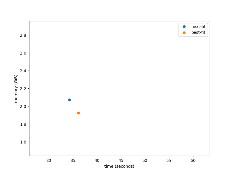
But that’s not the whole story. The best-fit memory allocator reduces fragmentation, packing allocations together more tightly. If we measure both time spent and memory used, we see there’s a trade-off here, with best-fit running slightly slower but using less memory:

But that’s not the whole story either. It would be, in a language with manual memory management, where the allocator has to deal with a sequence of malloc and free calls determined by the program. On the other hand, in a language with garbage collection, the GC gets to choose when memory is freed. By collecting more slowly, we free later, using more memory and less time. Adjusting the GC rate trades space and time.

So, in a GC’d language the performance of a program is not described by a single (space, time) pair, but by a curve of (space, time) pairs describing the available tradeoff. The way to make this tradeoff in OCaml is to adjust the space_overhead parameter from its default of 80. We ran the same benchmark with space_overhead varying from 20 to 320 (that is, from 1/4 to 4x its default value), giving us a more complete space/time curve for this benchmark. The benchmark is relatively noisy, but we can still see a separation between best-fit and next-fit:

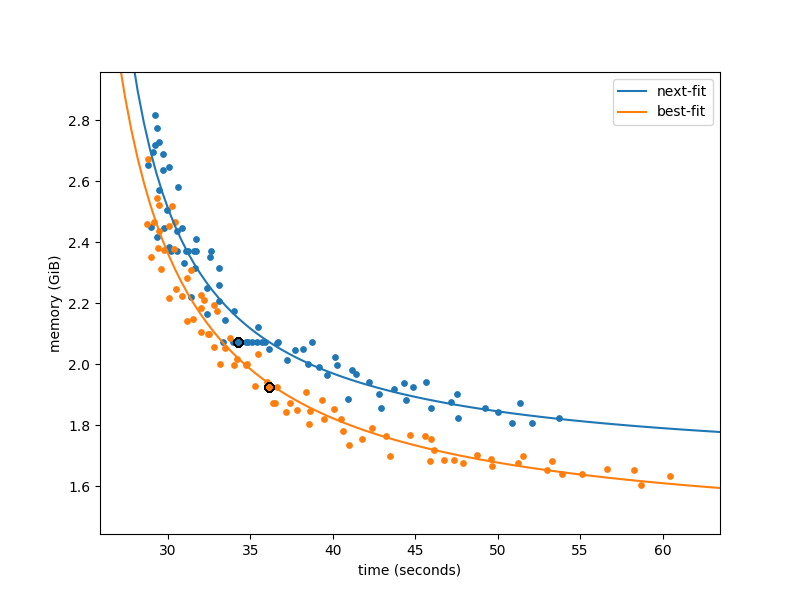
Here, best-fit handily beats next fit, whether optimising for time or space. Note that for every blue point there is an orange point below and left of it, likely with a different space_overhead value. (Also note that these numbers come from one of the benchmarks that best-fit performed the worst on.)

In the default configuration, best-fit picks a point on the curve that’s a bit further to the right than next-fit: it’s optimising more aggressively for space use than time spent. In hindsight, this is to be expected: internally, the space_overhead measure does not take into account fragmentation, so for a given space_overhead value best-fit will use less space than next-fit, as it fragments less.

That’s almost the whole story. There are just two questions left: what exactly do mean mean by “memory use” and where did the curves come from?

Measuring memory use

The y axis above is marked “memory use”. There are suprisingly many ways to measure memory use, and picking the wrong one can be misleading. The most obvious candidate is OCaml’s top_heap_size, available from Gc.stat. This can mislead for two reasons:

• It’s quantized: OCaml grows the heap in large chunks, so a minor improvement in memory use (e.g. 5-10%) often won’t affect top_heap_size at all.

• It’s an overestimate: Often, not all of the heap is used. The degree to which this occurs depends on the allocator.

Instead, the memory axis above shows Linux’s measurements of RSS (this is printed by /usr/bin/time, and is one of the columns in top). RSS is “resident set size”, the amount of actual physical RAM in use by the program. This is generally less than the amount allocated: Linux waits until memory is used before allocating RAM to it, so that the RAM can be used more usefully (e.g. as disk cache) in the meantime. (This behaviour is not the same thing as VM overcommit: Linux allocates RAM lazily regardless of the overcommit setting. If overcommit is disabled, it will only allow allocations if there’s enough RAM+swap to handle all of them being used simultaneously, but even in this case it will populate them lazily, preferring to use RAM as cache in the meantime).

The relationship between top_heap_size and RSS differs between allocators:

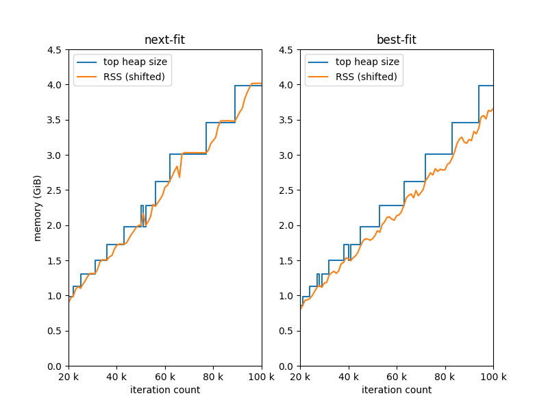
This graph shows the same benchmark run with different iteration counts. Each datapoint is a separate run of the program, whose memory use is larger with larger iteration counts. The RSS lines are shifted vertically to align at the left: without this change, the RSS lines are larger than the heap size because they also include binary size. The shifted RSS lines slightly exceed top heap size at the right of the graph, since not quite all of the memory allocated is heap (this happens on both but is more obvious on next-fit).

Notice that the next-fit allocator often uses all of the memory it allocates: when this allocator finds the large empty block at the end of the heap, it latches on and allocates from it until it’s empty and the entire allocated heap has been used. Best-fit, by contrast, manages to fit new allocations into holes in the heap, and only draws from the large empty block when it needs to. This means that the memory use is lower: even when the heap expands, best-fit does not cause more RAM to be used until it’s needed. In other words, there is an additional space improvement of switching to best-fit that does not show up in measurements of top_heap_size, which is why the first graph above plots memory as measured by RSS.

Modelling the major GC

The curves in the first graph above are derived by fitting a three-parameter model to the runtime and space usage data points. Here’s how that model is derived, and roughly what the parameters mean.

The time taken by major collection, under the standard but not-particularly-reasonable assumption that all cycles are the same, is (mark_time + sweep_time) * #cycles. Mark time is proportional to the size of live heap (a property of the program itself, independent of GC settings like space_overhead), and sweep time is proportional to the size of the live heap + G, the amount of garbage collected per cycle. This amount G is roughly the amount allocated, so the number of cycles is roughly the total allocations (another property of the program itself) divided by G.

The result is that the total runtime is roughly some affine linear function of (1/G), and the total heap size is roughly G plus a constant. That means that heap size is a function of runtime as follows:

H = 1/(t-a) * b + c

for three constants a, b, c. Fitting this 3-parameter model gives the curves in the original graph.

The parameters a, b and c have straightforward interpretations. a is the vertical asymptote, which is the minimum amount of time the program can take if it does no collection at all. This consists of the program code plus the allocator, so best-fit improves a by being faster to allocate. c is the horizontal asymptote, the minimum amount of space the program can use if it collects continuously. This consists of the live data plus any space lost to fragmentation, so best-fit improves c by fragmenting less. Finally, b determines the shape of the curve between the two asymptotes. This is broadly similar between the two allocators, since changing the allocator doesn’t strongly affect how fast marking and sweeping can be done (although stay tuned here, as there’s some work in progress on speeding up marking and sweeping with prefetching).

Conclusion

Switching allocators from next-fit to best-fit has made most programs faster and smaller, but it’s surprising how much work it took to be able to say that confidently!